5.3. TIN Surfaces

A TIN (Triangulated Irregular Network) surface models terrain or any 3D surface from a set of survey points. The surface is built using Delaunay triangulation and can display elevation contour lines.

5.3.1. Triangulation Algorithm

The triangulation engine uses the Bowyer-Watson incremental Delaunay algorithm (UTINTriangulation.pas), accessed through the ITINTriangulator interface for future algorithm swappability.

How Bowyer-Watson works:

Create a super-triangle that encloses all input points.
Insert points one at a time in randomised order (Fisher-Yates shuffle).
For each inserted point, find all existing triangles whose circumcircle contains the new point (these are the “bad” triangles).
Remove the bad triangles, leaving a star-shaped polygonal hole.
Re-triangulate the hole by connecting the new point to all edges of the hole boundary.
After all points are inserted, remove any triangles that share vertices with the original super-triangle.

Performance optimisations for large point sets (100K+):

Randomised insertion — prevents worst-case O(n²) behaviour on ordered point sets (e.g. grid scans, sorted CSV files).
Flat-grid spatial index — triangles are assigned to grid cells based on their circumcircle AABB. Point insertion only checks triangles in nearby cells instead of scanning all triangles.
Auto-scaling grid — resolution scales as sqrt(N) cells per axis, clamped to [16..1024], balancing cell occupancy and lookup cost.
Overall complexity — O(n√n) average, compared to O(n²) without the spatial index.

5.3.2. Creating a Surface

Use any of the following methods:

Civil › Surfaces › Create Surface or ribbon button Create Srf
Type CREATESURFACE (alias CS) in the command line
Right-click Surfaces in the Civil Toolspace and choose Create Surface…

A surface with an auto-generated name (Surface_1, Surface_2, …) is created. If survey points already exist in the drawing they are triangulated automatically; otherwise an empty surface definition is created.

5.3.3. Adding Data to a Surface

An empty surface can be populated in several ways, matching the AutoCAD Civil 3D workflow:

From survey points:

Type ADDSURFACEPOINTS (alias ASP) and enter the surface name. All survey points in the drawing are collected and the TIN is built.
Or right-click the surface name in the Civil Toolspace and choose Add Survey Points.

From drawing objects (3DFaces, Lines, Polylines, etc.):

Select the source entities on the canvas.
Type ADDSURFACEENTITIES (alias ASE). If only one surface exists it is used automatically; otherwise you are prompted for the name.

Supported entity types:

Entity	How it contributes
3DFace	3 or 4 corner vertices loaded as TIN triangles directly (no re-triangulation). Quads are split into two triangles.
Line	Both endpoints contribute as TIN data points.
Polyline / Spline	All vertices contribute as TIN data points.
Point / Survey Point	Position contributes as a TIN data point.

When the selection contains only 3DFaces, triangles are loaded verbatim (preserving the original mesh topology). When non-face entities are present, all collected vertices are triangulated using Delaunay.

You can also right-click a surface name in the Civil Toolspace and choose Add Drawing Objects… to add the currently selected entities.

Rebuilding:

After adding or moving survey points, type REBUILDSURFACE (alias RS) and enter the surface name to re-triangulate from the current point positions.

5.3.4. Surface Display & Styles

Surface display is controlled through Surface Styles — named presets that bundle all visual settings into one reusable object.

Each surface references a style by name via the StyleName property in the Object Inspector. Three built-in presets are provided:

Style	Description
Standard	Shows triangles, contours, boundaries, and contour labels.
Triangles & Contours	Triangles and contours visible, boundary hidden.
Contours Only	Only contour lines and labels.
Elevation Banding	Contours and elevation bands visible.
Empty	All components hidden. Use to suppress a surface from display without deleting it.

Open the Surface Style Editor via:

Format > Surface Styles…
Right-click a surface in the Civil Toolspace > Surface Style…

The editor has 3 property tabs (Border & Triangles, Contours, Contour Labels) plus a style list for creating/editing/deleting styles.

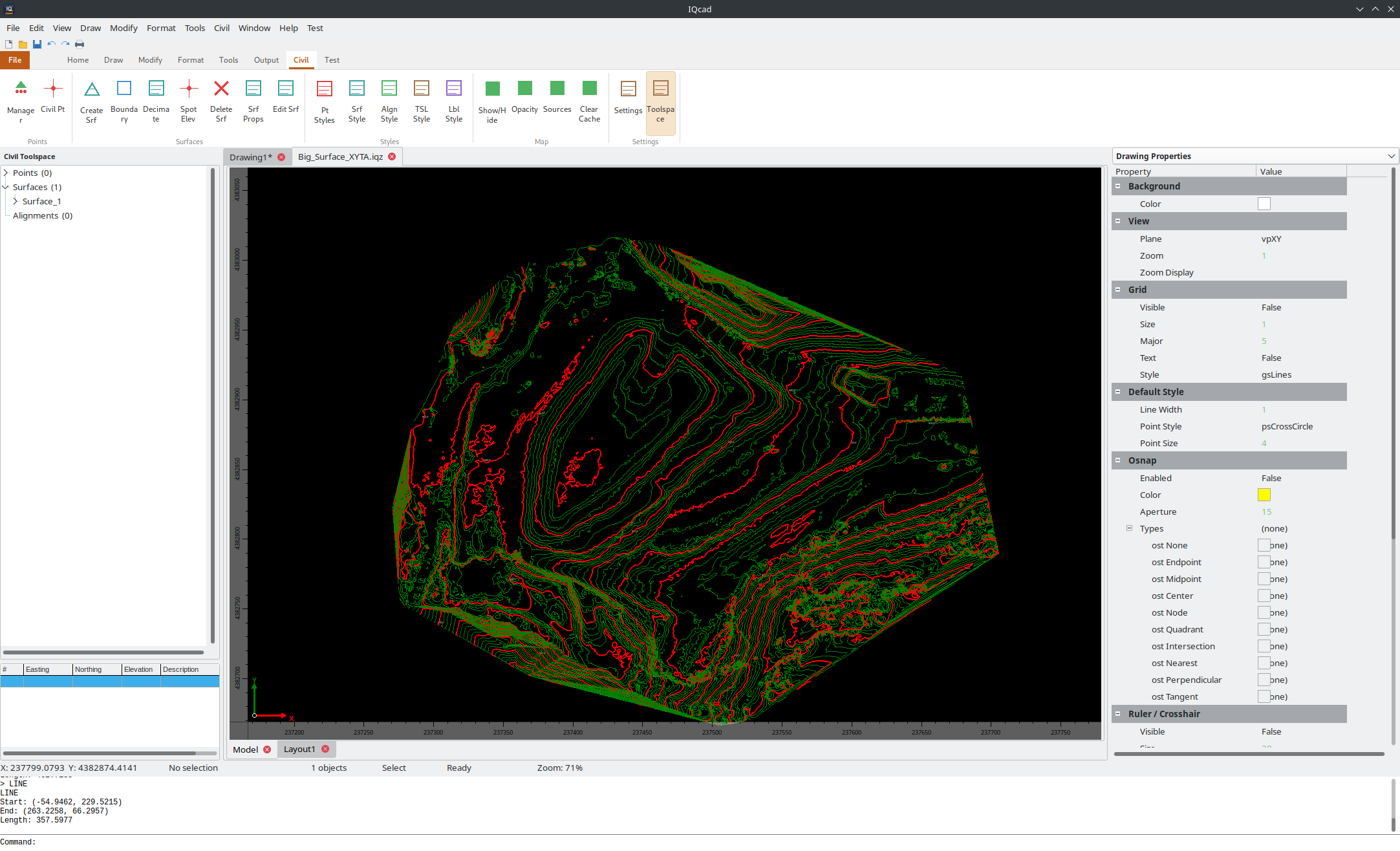
../../_images/surface_example.png — A TIN surface with contour lines and elevation labels.

Style properties cover 5 groups (~35 settings): border (visibility, colour, weight), triangles (visibility, colour, weight), contours (visibility, major/ minor interval, colours, weights, smoothing, base elevation), contour labels (visibility, interval, text height, precision, prefix/suffix, colour, font, background mask, uphill-readable rotation), and points (visibility, colour, size).

Contour labels are placed automatically along contour polylines with:

Interval-based placement with collision avoidance
Uphill-readable rotation — label text top faces uphill
Optional background mask for readability
Manual label placement via user-placed points

Changing the style immediately regenerates contours if the interval or smoothing parameters differ from the cached values.

5.3.4.1. Contour Generation Algorithm

Edge marching — for each triangle, for each contour elevation within its Z range, find the two edge crossings by linear interpolation. Each crossing produces a 2-point segment.
Segment joining — chain the 2-point segments into continuous polylines by matching endpoints. Uses a spatial hash table with linked-list chaining for O(1) endpoint lookup (Fibonacci hashing, QUANT = 1e-6, table size = next power of 2 ≥ 2×N segments). This replaces the naive O(s²) greedy scan and makes joining nearly instant even for millions of segments.
Chaikin smoothing — apply corner-cutting subdivision (ContourSmoothing passes) to produce smooth curves.

Lazy generation for large surfaces. When LoadTINData receives more than 100 000 triangles, contour generation is deferred: ShowContours is set to False and contours are only computed when the user first enables ShowContours via the Object Inspector. This prevents the UI from blocking during large LandXML imports.

5.3.5. Boundaries

Boundaries clip the TIN to a specific area. Use Civil › Surfaces › Add Boundary or the command ADDSURFACEBOUNDARY (alias ASB) to add an outer boundary or hole boundary to a surface.

Outer boundary — triangles whose centroids fall outside the polygon are removed.
Hole boundary — triangles whose centroids fall inside the polygon are removed.

5.3.6. Surface Statistics

The Object Inspector shows the following read-only statistics:

PointCount — number of TIN vertices.
TriangleCount — number of Delaunay triangles.
SurfaceArea — total 3D surface area. For surfaces exceeding 500 000 triangles the area is estimated by sampling every N-th triangle and extrapolating, so the calculation remains instant.
MinElevation / MaxElevation — elevation range.

These statistics are also displayed in the Civil Toolspace grid when the surface node is selected.

5.3.7. Elevation Query

The surface provides a GetElevationAt(X, Y) method that returns the interpolated Z elevation at any (X, Y) position on the TIN. Interpolation uses barycentric coordinates inside the triangle that contains the query point — no re-triangulation is needed. This method is used internally by the greedy decimation algorithm and can be called from scripts.

5.3.8. Elevation Tracker

The Elevation Tracker is a live readout of terrain elevation under the mouse cursor, as you move it over the canvas — no picking or clicking required. Toggle it from the Civil ribbon or menu (the button stays pressed while active), or type ELEVTRACK in the command line. While on, moving the mouse shows a small overlay box near the cursor listing the current elevation of every visible surface under that point (a surface hidden by its layer or style is skipped); if several surfaces overlap, all their elevations are listed together so you can compare them at a glance. When more surfaces are under the cursor than the overlay can comfortably show, the extra rows collapse into a “+*N* more…” line.

Point clouds. A second, independent toggle — PCELEVTRACK (also on the Point Cloud ribbon tab and menu) — extends the same readout to loaded point clouds: for each visible cloud, it reports the elevation of the single nearest point to the cursor within a small search radius (no averaging or interpolation — a real measured point), sorted with the surface hits in one combined overlay. A cloud with no point close enough to the cursor contributes no row. Turning either tracker off only clears its own rows; the other keeps working independently. See Point Clouds for more on point cloud display.

5.3.9. Performance & Rendering

Large surfaces (millions of triangles) use several automatic optimisations to keep the editor responsive:

Triangle sub-sampling — when the TIN exceeds 500 000 triangles, only every N-th triangle is drawn (MAX_DRAW_TRIANGLES = 500 000). This caps GDI draw calls and keeps panning/zooming smooth.
Viewport culling — triangles whose three vertices all fall outside the same viewport edge (left, right, top, or bottom) are skipped entirely.
Sub-pixel culling — triangles that project to a single screen pixel (all three screen coordinates identical) are not drawn.
Lazy contour generation — when LoadTINData receives more than 100 000 triangles (e.g. during a LandXML import), ShowContours is set to False and contours are only computed when the user first enables them via the Object Inspector. This prevents the UI from blocking.
Surface area sampling — for surfaces exceeding 500 000 triangles the 3D surface area statistic is computed by sampling rather than iterating every triangle.

No user configuration is required — all thresholds are applied automatically.

5.3.10. IQML Streaming Save

Surface entities (and all other entity types) are serialised to IQML using a streaming writer that writes directly to a text file instead of building an in-memory DOM tree. This eliminates millions of XML node allocations and keeps memory usage constant regardless of drawing size.

Drawings with 1 000 000+ entities save in seconds instead of minutes.
The IQML file format is identical — streaming is transparent.

5.3.11. Decimating (Simplifying) a Surface

Dense TIN meshes — for example from drone photogrammetry, LiDAR, or large LandXML imports — can contain millions of triangles. The Decimate Surface command reduces the TIN to a much smaller mesh while preserving the surface shape within a user-specified vertical tolerance.

Use any of the following methods:

Civil › Surfaces › Decimate Surface…
Ribbon button Decimate in the Surfaces pane of the Civil tab
Type DECIMATESURFACE (alias DS) in the command line

You will be prompted for:

Surface name — auto-selected if only one surface exists.
Max elevation tolerance — the maximum allowed vertical error (in drawing units, e.g. 0.05 for 5 cm).

5.3.11.1. Decimation Algorithms

The system automatically selects the best algorithm based on the number of input points (threshold: 100 000 points).

Algorithm A — Grid-Based Decimation (> 100K points)

O(n) single-pass algorithm designed for very large surfaces (millions of points). Completes in seconds even for 4M+ points.

Bounding box pass — compute the XY extent and simultaneously track the 4 boundary extreme points (min-X, max-X, min-Y, max-Y). These replace an expensive O(n log n) convex hull computation.
Grid setup — divide the XY extent into an aspect-ratio-aware grid. Grid resolution: N / 50 cells (roughly 2% of input), capped at 50 000 cells to keep the subsequent triangulation fast.
Cell statistics pass — single pass over all N points. For each grid cell, track the point with the minimum Z and the maximum Z.
Point selection — for each occupied cell:
- Always keep the max-Z point (preserves terrain highs).
- Also keep the min-Z point if the cell’s Z range exceeds the tolerance (preserves valleys, ridges, and terrain features).
Triangulation — Bowyer-Watson on the reduced point set (typically 30K–80K points).

Algorithm B — Greedy-Insertion Refinement (≤ 100K points)

Higher-quality iterative algorithm where each inserted point is chosen to maximise error reduction.

Seed — start with a triangulation of the convex hull corners only.
Error computation — for every omitted point, compute its vertical error against the current (coarse) TIN surface using a grid-accelerated triangle lookup for Z interpolation.
Batch insertion — pop a batch of the highest-error points from a binary max-heap and insert them all at once, then re-triangulate. Adaptive batch sizes (20–500 points) scale with remaining count.
Error update — recompute errors for all remaining omitted points against the updated TIN. O(n) bottom-up heap rebuild.
Stop — repeat until max error ≤ tolerance, or MaxPoints reached.

Typical results:

Input	Algorithm	Tolerance	Time	Reduction
4 235 712 pts	Grid	0.10 m	< 5 sec	~99%
500 000 pts	Grid	0.05 m	< 2 sec	~97%
50 000 pts	Greedy	0.02 m	~10 sec	~70%

After decimation the contours and boundaries are automatically regenerated.

5.3.12. Deleting a Surface

Use Civil › Surfaces › Delete Surface or type DELETESURFACE in the command line and enter the surface name.

5.3.13. Importing Large Surfaces (LandXML Fast Path)

LandXML files ≥ 10 MB are imported using a streaming fast path that bypasses DOM parsing entirely:

Line-by-line reader (ULandXMLFastReader) — reads the file sequentially without building an XML DOM tree in memory.
Direct array ID→index mapping — O(1) point ID lookup instead of TFPGMap sorted-list binary search.
Inline number parsing — float and integer values are parsed in-place without allocating TStringList per XML element.
Memory — O(points + triangles) only; doubling array growth for amortised O(1) insertions.

The fast path is activated automatically and transparent to the user — the import dialog and workflow are identical. Small files continue to use the standard DOM-based path.

5.3.14. Exporting Surfaces

DXF: triangles export as 3DFACE entities; contour lines export as 3D polylines on dedicated layers (<Name>-Contour-Major and <Name>-Contour-Minor).
LandXML: surfaces export as <Surface>/<Definition surfType="TIN"> with <Pnts> and <Faces> elements.
IQML: full round-trip including TIN data, boundaries, contour settings, and source group names.

5.3.15. Cross-Sections from a DEM

Existing-ground cross-sections can be taken directly from a raster DEM — no triangulation or survey points required. The workflow combines three commands and reuses the standard section-sheet pipeline.

1. Import the DEM. IMPORTDEM (alias IDEM) reads a GeoTIFF elevation raster (.tif) and adds it to the drawing as a grid-backed surface. The reader is native — it handles uncompressed, Deflate, and LZW compression; single-band Float32 or Int16 samples; and both strip and tiled layouts — and georeferences the DEM from the GeoTIFF’s own tags (model tiepoint, pixel scale, and CRS), so no world file or external conversion is needed. NoData values, voids, and non-finite cells are treated as gaps: the surface returns no elevation there rather than fabricating ground.

A grid-backed DEM surface answers elevation queries by bilinear interpolation directly on the raster grid; it never builds a TIN. Because it still behaves as a surface, it is sampled by section sheets, reported in cut/fill, and picked from the canvas exactly like a triangulated surface. It is drawn as its extent rectangle and is persisted in the drawing by storing its source path; on reopen the .tif is re-decoded automatically (a warning is shown if the file has been moved).

Note

The DEM’s CRS is reported on import but not reprojected. The DEM, the alignment, and any point cloud must already share one projected coordinate system, or the sections will be sampled at the wrong location.

2. Build a comparison surface from the point cloud. To validate the DEM against survey data, CLOUDSURFACE (alias CLS) turns a loaded point cloud into a second grid surface. It bins the cloud’s ground-classified points (LAS class 2) into a regular grid, keeping the lowest Z in each cell to estimate bare earth, and names the result Cloud_<name>. Cell size defaults to roughly twice the average point spacing. Empty cells stay void, so the comparison surface never invents ground from a single stray return. If the cloud has no ground classification, CLOUDSURFACE falls back to all points and suggests running PCGROUND first to classify ground for a cleaner bare-earth result.

3. Cut the sections. Run CREATESECTIONSHEET, pick the alignment, then select both the DEM surface and the Cloud_* surface (the cut/fill prompts appear only when two or more surfaces are chosen). Each station then shows a DEM ground line and a cloud ground line, with cut/fill reported between them — close agreement confirms the DEM, while large gaps flag DEM voids, interpolation artefacts, or vegetation left in the cloud.

Orthophoto backdrop (optional). A georeferenced orthophoto can be draped under the plan for context with IMAGEATTACH, which reads the image’s world file (.jgw/.tfw) for placement, followed by DRAWORDER → Back to send it beneath the vector geometry. Large JPEG orthophotos are decoded at reduced scale, so a gigapixel image displays as a backdrop instead of a white placeholder.

5.3.16. Comparing Surfaces (Surface Differencing)

Two surfaces — or a surface and an as-built point cloud — can be compared to produce a difference (diff) surface whose elevation at every point is the vertical deviation dz between them. This is the basis for earthwork quality control: comparing a theoretical (design) surface against a built or surveyed one shows exactly where material is missing (fill) or in excess (cut), colour-banded by how far each area strays from tolerance.

Two commands open the same Compare Surfaces dialog:

SURFDIFF — compare two TIN surfaces. Civil › Surfaces › Compare Surfaces…, or the Compare Two Surfaces ribbon button on the Civil tab.
PCDIFF — compare a surface against a loaded point cloud. The Compare ribbon button in the Point Cloud pane.

In the dialog:

Surface A (theoretical) and Source B (built) — pick the two inputs. A is always a TIN surface; B is a surface (SURFDIFF) or a point cloud (PCDIFF).
Cell size (m) — the diff is computed on a regular grid; smaller cells give finer resolution but more triangles. A live preview reports the overlap extent, the resulting cell count and an estimated build time, and refuses to run if the two inputs do not overlap in plan or the cell count exceeds the safety cap.
Tolerance (m) — deviations within ±tolerance are treated as on target (the neutral band). Default 0.20 m.
Max deviation (m) — the outer limit of the colour ramp; areas beyond it saturate to the end colours. Leave 0 to auto-set (5 × tolerance).
Sign convention — A − B (positive = under-build, fill needed) or B − A (positive = over-build). The note under the combo and the colour swatch update live.
PC reducer (point-cloud compare only) — how multiple returns in one cell collapse to a single ground value: Median (recommended for noisy scans), Minimum or Mean.
Insert as named entity — add the result to the drawing as DIFF_<A>-vs-<B> (clear it for a statistics-only run).
Show statistics after compare — pop up a summary of valid samples, min/max/mean/RMS dz and cut/fill volumes when the compare finishes.

The result surface carries a deviation-banded style (blue → red ramp by default): a neutral band around zero and symmetric cut/fill bands out to the max deviation. It behaves like any surface — pick it, restyle it, sample it — and is saved in the drawing (IQML) together with its comparison provenance (both source names, sign, tolerance, cell size) so the volume report below still works even after the source surfaces are gone.

5.3.17. Earthwork Volume Report

The Volume Report turns a comparison (diff) surface into a printable HTML earthwork report — cut, fill and net volumes, the areas they cover, deviation statistics, and a per-band breakdown. Every figure is integrated directly from the diff surface’s own triangulation (each triangle contributes its 2D-projected area × its mean deviation), so the report is self-contained and works on any saved diff surface without the original inputs.

Open it via:

Civil › Surfaces › Volume Report…
The Earthwork Volume Report ribbon button on the Civil tab
The Volume Report action on a selected diff surface in the Object Inspector
The View the full volume report? prompt offered right after a compare (when Show statistics after compare is on and the diff was inserted)
Command VOLUMEREPORT (alias VOLREPORT)

When no surface is passed, the command uses the single selected diff surface, or — when several diff surfaces exist — prompts you to choose one. A surface that is not a comparison surface is rejected with a message. The report opens in the system browser, from where it can be printed or saved to PDF.

The report has four sections:

Summary — the diff surface name, both source names, sign convention, compare timestamp, tolerance, cell size, and grid coverage (valid vs total samples).
Volumes — cut volume, fill volume, net volume (fill − cut), and the cut / fill / total areas, in m³ and m².
Deviation statistics — minimum, maximum, mean and RMS dz. These use the compare-time grid samples when available, otherwise the TIN nodes.
Deviation bands — one row per colour band, each with its dz range, a colour swatch, its area, its signed volume, and its share of the total area. The band ranges and colours are read from the surface’s on-screen style, so the table matches the map exactly.

Note

Cut and fill are both reported as positive magnitudes; net = fill − cut (a negative net means net cut). The band volumes are signed (negative for cut bands), so they sum to the net volume, while the band areas sum to the total area.

5.3.18. Balancing Volumes

Balance Volumes edits a design surface so that its cut/fill against existing ground hits a target — most often net zero for a pad, or a given fill volume for a landfill or stockpile. The design surface itself is not changed: the edited copy is inserted as a new surface named BAL_<design>, so you can run the tool again with another target.

Open it via Civil › Surfaces › Balance Volumes…, the Civil ribbon Surfaces menu, or the command SURFBALANCE (alias BALANCEVOLUMES). The drawing needs at least two surfaces.

Existing ground / Design — the two surfaces. Only the design moves.
Region of the edit — Whole overlap, or Inside polyline to confine the edit to a closed polyline (a pad outline, a landfill plateau).
Transition to untouched design — how the edit fades out beyond the inner polyline: None (a step, built as a 5 cm taper), To polyline (linear fade out to a second, outer polyline — for a pad use the daylight line) or Width (linear fade over the given distance).
Method — Shift design up/down raises or lowers the region by one value dZ (pads). Scale thickness, toe fixed multiplies the thickness between design and existing ground by a factor K, so the design stays pinned wherever it already meets the ground (landfills, stockpiles, ponds). Scaling cannot balance a surface that has both cut and fill — use Shift there.
Target — the measure and its value in m³: Net (fill − cut; 0 = balanced), Cut or Fill.
Fill factor — multiplies the fill before it is compared with the target or the cut: above 1 for shrinkage (more bank material per placed m³), below 1 for swell. The cut is never factored.
Cell — the sampling grid, as for SURFDIFF.

Press Compute: the table shows the current cut, fill, factored fill and net, the solved dZ or K, and the predicted volumes after the edit. All volumes are totals over the overlap of both surfaces — the region only confines the edit. Apply inserts the new surface (with the design’s style), recomputes the volumes on it and shows them next to the prediction. Report the recomputed figures: the prediction is made on the sampling grid, the new surface is a TIN, and on a coarse design surface the two can differ by a little along the region edge. Run Compare Surfaces on the new surface against existing ground for the full volume report.

Changing any input after a compute clears the prediction and disables Apply until you compute again. When the target cannot be reached the dialog says so and shows the closest result; Apply then asks for confirmation.

5.3.19. Surface Editing Commands

IQcad provides interactive TIN editing commands for modifying a surface after it has been created. All surface edit operations are logged and can be undone.

Command	Alias	Description
`SURFADDPOINT`	`SAP`	Add a single point to the surface TIN interactively.
`SURFDELETEPOINT`	`SDP`	Delete a point from the surface TIN.
`SURFMOVEPOINT`	`SMP`	Move a surface TIN point to a new position.
`SURFMODIFYELEV`	`SME`	Modify the elevation of a surface point.
`SURFSWAPEDGE`	`SSE`	Swap a TIN edge between two adjacent triangles.
`SURFADDLINE`	`SAL`	Force an edge between two points in the TIN (breakline).
`SURFDELETELINE`	`SDL`	Remove a TIN edge.
`SURFDELETELONGEDGES`	`SDLE`	Delete every TIN edge longer than a threshold you type — the standard way to trim the long slivers a convex hull throws around a concave survey.
`SURFHIDETRI`	`SHT`	Hide triangles by clicking inside them; right-click to finish. See Hiding and Restoring Triangles below.
`SURFSHOWTRI`	`SWT`	Restore every hidden triangle on the picked surface.
`SURFRAISELOWER`	`SRL`	Raise or lower the entire surface by a specified elevation offset.
`SURFUNDO`	(none)	Undo the last surface edit operation.
`SURFCLEAREDITS`	`SCE`	Clear the surface edit log.
`SURFLISTEDITS`	`SLE`	List all surface edit operations performed since the last clear.
`SURFADDBREAKLINE`	`SAB`	Convert the selected polyline(s) into surface breaklines (forced edges that the TIN must respect). If nothing is selected when the command runs, you are prompted to pick polylines on the canvas.

5.3.20. Hiding and Restoring Triangles

Triangulation is convex: a TIN built from a survey that is not convex — a road corridor, a river bank, a site with a re-entrant boundary — always spans ground that was never surveyed. A boundary clips that away (see Boundaries above); hiding individual triangles handles the cases a boundary cannot express, such as a single bad face over a building or a gap between two survey blocks.

SURFHIDETRI (alias SHT) runs as a loop:

Pick the surface if more than one is in the drawing.
Click inside a triangle to hide it. The face disappears from the surface display, contours regenerate around it, and the command line reports the count hidden in this run and in total.
Right-click to finish.

A hidden triangle is kept, not deleted. It stays in the surface’s edit log, is excluded from the displayed and contoured surface, and can be brought back at any time:

SURFSHOWTRI (alias SWT) restores every hidden triangle on the picked surface at once and reports how many came back.
SURFUNDO steps back through hide operations like any other surface edit.

Note

Hiding faces changes what the surface displays, not the points it was built from. Elevation queries and volume calculations use the surface as displayed, so hiding a face over a building removes it from the volume too — which is normally what you want, and is why the operation is logged rather than destructive.

Civil 3D stores hidden faces the same way, in the triangulation itself. Surfaces read from a Civil 3D DWG come in with their hidden faces already flagged, and faces deleted there are dropped on read.

5.3.21. Breaklines

A breakline is a polyline whose segments are forced into the TIN as constrained edges. Use them to model break-of-slope features — top of bank, bottom of bank, pavement edge, ridge, swale — that the triangulation must follow. A constrained edge is never flipped by a later swap-edge or delete-line operation.

Adding a breakline:

Draw a polyline along the feature.
Select the polyline.
Run SURFADDBREAKLINE (alias SAB), or right-click the surface’s Definition node in the Civil Prospector and choose Add Breakline....

The surface stores its own copy of the polyline geometry, so editing or deleting the source polyline afterwards leaves the breakline intact. Each vertex is snapped to an existing TIN point within 1 cm or inserted into the triangulation if no nearby point exists; the segments between consecutive vertices are then forced as constrained edges.

The Civil Prospector tree shows a Breaklines (N) node under each surface’s Definition. Right-click an entry to Delete it. Removing a breakline drops its constraints — points it inserted remain in the TIN, but the triangulation is free to flip those edges again.

Visual style is controlled by the Breaklines tab in the Surface Style editor: visible toggle, color, weight, linetype, linetype scale. The default colour is magenta so breaklines stand out from triangle wireframe and boundary edges. When the Civil object-layer system is active, the breakline geometry is placed on the dedicated Surface/Breakline component layer (default suffix BRKL → C-TOPO-BRKL).

5.3.22. Spot Elevations

The Spot Elevation tool (SPOTELEV, alias SE) places an elevation label at a clicked point on a surface. The tool queries the TIN to interpolate the Z value at the click position and displays it as a text annotation on the canvas.

Access via:

Civil > Surfaces > Spot Elevation
Ribbon button Spot Elev on the Civil tab
Command SPOTELEV (alias SE)

5.3.23. Contour Label Placement

The Add Contour Labels command (ADDCONTOURLABEL, alias ACL) places elevation labels along contour lines of a surface. Labels are positioned automatically with collision avoidance and uphill-readable rotation.